Alert!
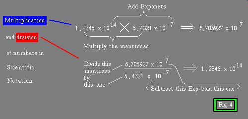
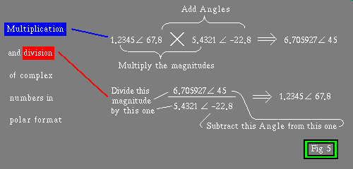
There is a rather obvious booboo in the audio, starting at 24:21
(24 minutes, and 21 seconds) and ending at 24:38 just pay attention
to the wording in figure five, and you'll stay on the right track.
Sorry about this, I intend to annotate minor errors in the audio
in these Alerts at the beginning of the page, and defer editing
the actual audio to one single massive project later after I discover
all the mistakes. This may seem like a burden to you, but if you think
about it for a moment you, or atleast most of you will appreciate this
strategy, as it avoids the necessity, of re-downloading large mp3 files
everytime I make some small incremental change.
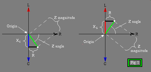
This lesson assumes familiarity with your scientific calculator's
"Polar <--to--> Rectangular"
coordinate conversion facility, if you feel you are weak in this area, start
the audio download, and get out the owners manual for your scientific
calculator, and learn how to make these conversions. With any luck, just as
you get the hang of doing this the audio will have arrived, and you will be
ready for it without missing a step.
Click the "Audio discussion" link now, then
read on while it's downloading. When it
arrives, come back here, to start, and as I
progress through the audio discussion, I'll
instruct you to proceed from one pictorial
to the next, like a slide presentation
013_Vector_math.mp3 Audio lecture
on Phasor Diagrams 14.67 meg
Proving to your self, you can do it.
Your Notes:
First I repeat the examples in the graphics, here so that you can
scoop them up into your favorite editor, and hack away at them.
You should be trying to edit them into such a form that you can
leave room in what will become a printed version of what we in the
good ole days called home work. Your assignment is to do these
examples, and see if your results are atleast close to mine.
don't expect exact matching results, many of these examples exceed
most scientific calculators arithmetic precision, so the results
may be no better than
slide rule
accuracy. I have an HP15C and others, they disagree with each other,
this is not surprising, and if you are the trusting type, it's time
you became a little less so, just because the calculator says it's
so, or the computer says it's so, doesn't mean the firmware in the
calculator, or the software in the computer is flawless,
additionally, the end user is often unaware of the implications of
the math he or she is trying to force the software to work out.
This often looses so much precision, that the results obtained, are
utterly worthless, this happens frequently in spreadsheet
applications, and millions of dollars are lost because the computer
said go for it, in a what if scenario, when the precision was lost
in the noise of the sixtieth decimal place, and the user had no
idea the spread sheet was adding up garbage.
Then I will repeate this same information, sprinkling in hopefully
useful commentary, about each of the phases.
-------------------------------------------
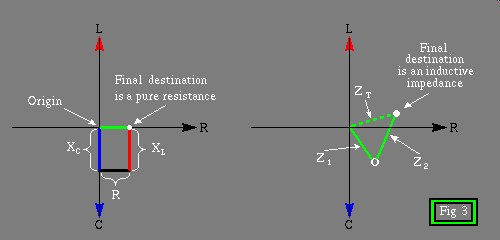
fig 3 Solve for series impedance
(-10y, 0x) + (0y, 6x) + (10y, 0x)
Result
0y, 6x or 6 @ 0 deg
-------------------------------------------
fig 7 Solve for parallel impedance
1 @ 0 deg
----------------------------
1 @ 0 deg 1 @ 0 deg
------------- + ------------
10 @ 90 deg 10 @ -90 deg
0 y , 1 x
----------------------------
(-0.1y, 0x) + (0.1y, 0x)
Result
division by zero
1 @ 0 deg
--------------------------------
1 @ 0 deg 1 @ 0 deg
----------- + ----------------
10 @ 90 deg 9.9999 @ -90 deg
1 y , 0 x
-----------------------------------
(-0,1 y , 0 x) + (0,100001 y , 0 x)
Result
-1000000y, 0 x or 1000000 @ -90 deg
-------------------------------------------
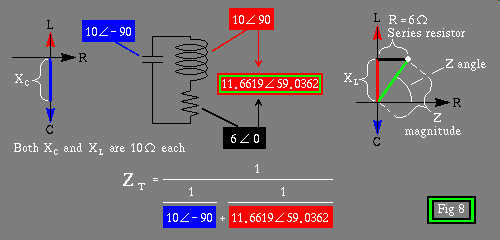
fig 8 Solve for series parallel impedance
Step one: solve for the series
resistor and inductor
6 ohm pure resistance + plus 10 ohm
inductive reactance
(0 y , 6.0 x) + (10.0 y , 0 x)
= (10.0 y , 6.0 x)
Step two: Convert the series impedance of
the inductor, resistor combination into
Polar coordinates suitable for solving
for the reciprocal. Note: taking the
reciprocal is essentially division.
11.6619 @ 59.0362 degrees
Step three: Now we set up the rest of the
problem to solve for the parallel
combination impedance of the capacitor,
and the series, combination of the
resistor, and inductor.
1 @ 0 deg
--------------------------------------
1 @ 0 deg 1 @ 0 deg
-------------- + ---------------------
10 @ -90 deg 11.6619 @ 59.0362 deg
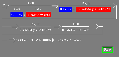
fig 9 This problem continues
Step four: solving for the two lower
reciprocal terms yields
1 @ 0 deg
-----------------------------------------
0.1 @ 90 deg + 0.0857493 @ -59.0362 deg
Step five: convert those two terms back
to Rectangular I.E. Y,X coordinate pairs
suitable for addition
0 y , 1 x
--------------------------------------
(0.1y, 0x) + (-0.0735294y, 0.0441177x)
Step six: compute the coordinate pair sum
of the two bottom terms
0 y , 1 x
--------------------------------------
(0.0264706y, 0.0441177x)
Step seven: convert back to Polar, eg.
Magnitude, and Angle to get it into a
form suitable for division
1 @ 0 deg
--------------------------
0.0514496 @ 30.9637
Step eight: carry out the division, that
is solve the last reciprocal
Result is 19.4364 @ -30.9637 deg
or in rectangular form the same
Result is -9.9999y, 16.666x
-------------------------------------------
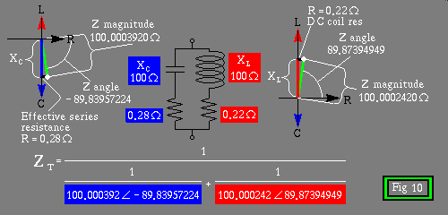
fig 10 Solve for series parallel impedance
Step one: solve for the inductor with its
inherent series coil resistance
0.22 ohm pure resistance + plus 100 ohm
inductive reactance
(100 y , 0 x) + (0 y , 0.22 x)
= (100 y , 0.22 x)
Step two: Convert the series impedance of
the inductor, resistance combination into
Polar coordinates suitable for solving
for the reciprocal. Note: taking the
reciprocal is essentially division.
100.000242 @ 89.87394949 degrees
Step three: solve for the capacitor with
its ESR, "effective series resistance"
0.28 ohm pure resistance + plus 100 ohm
capacitive reactance
(-100 y , 0 x) + (0 y , 0.28 x)
= (-100 y , 0.28 x)
Step four: Convert the series impedance
of the capacitor, ESR combination into
Polar coordinates suitable for solving
for the reciprocal.
100.000392 @ -89.83957224 degrees
Step five: Now we set up the rest of the
problem to solve for the parallel
combination impedance of the capacitor/w,
ESR, and the coil/w inherent series coil
resistance
1 @ 0 deg
-----------------------------------------
/ 1 @ 0 deg |
| ----------------------------- --+--
\ 100.000392 @ -89.83957224 deg |
1 @ 0 deg \
----------------------------- |
100.000242 @ 89.87394949 deg /
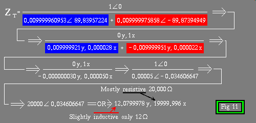
fig 11 This problem continues
Step six: solving for the two lower
reciprocal terms yields
1 @ 0 deg
-----------------------------------------
( 0.009999960953 @ 89.83957224 deg +
0.009999975858 @ -89.87394949 deg )
Step seven: convert those two terms back
to Rectangular I.E. Y,X coordinate pairs
suitable for addition
0 y , 1 x
--------------------------------------
( 0.009999921 y , 0.000028 x +
-0.009999951 y , 0.000022 x )
Step eight: compute the coordinate pair
sum of the two bottom terms
0 y , 1 x
--------------------------------------
-0.000000030 y , 0.000050 x
Step nine: convert back to Polar, eg.
Magnitude, and Angle to get it into a
form suitable for division
1 @ 0 deg
--------------------------
0.00005 @ -0.034606647
Step ten: carry out the division, that
is solve the last reciprocal
Result is 20000 @ 0.034606647 deg
or in rectangular form the same
Result is 12.0799978y, 19999.996x
-------------------------------------------
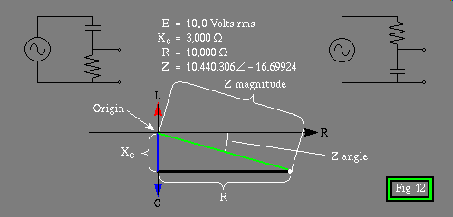
fig 12 To solve for AC voltage, "E" across
a resistor and across the series
capacitor, you need to solve for
current, "I" to do this, you need
to solve for total impedance, "Z"
Er = R I Egen
I = ---------- Zt = Xc + R
Ec = Xc I Zt
Knowns:
Egen = 10.0 volts rms
Xc = 3000 ohm @ -90 deg
R = 10000 ohm @ 0 deg
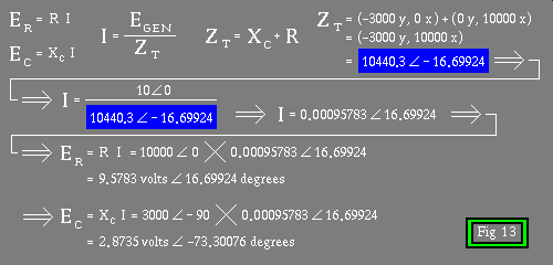
fig 13 This problem continues
Step one: solve for the total impedance
Zt = (-3000 y , 0 x) + (0 y , 10000 x)
= (-3000 y , 10000 x)
Step two: use Zt to solve for the current
Egen (0 y , 10 x)
I = ------- = ---------------------
Zt (-3000 y , 10000 x)
10 @ 0 deg
= -------------------------
10440.3 @ -16.69924 deg
= 0.00095783 @ 16.69924 deg
Step three: use I to solve for the
voltage drop across the resistor
Er = R I
= (10000 @ 0) x (0.00095783 @ 16.69924)
Result: Er = 9.5783 volts @ 16.69924 deg
Step four: use I to solve for the
voltage drop across the capacitor
Ec = Xc I
= (3000 @ -90) x (0.00095783 @ 16.69924)
Result: Ec = 2.8735 volts @ -73.30076 deg
-------------------------------------------
As promised I now repeate the above, so that I can add interesting
commentary about issues involved in setting up, and solving
problems in vertor algebra.
Vector Addition:
In fig 3 we simply Walk the Walk that is, we aim our selves
in the direction starting at the origin of a cartesian coodinate
plane and walk in the direction called out by the arithmetic
sign ( + or - ) in
either of two axis, rise, the Y axis, or run, the X axis.
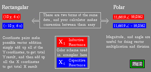
To accomplish this in simple arithmetic, the vectors must be in
rectangular form, that is, coordinate pairs, a rise/run
combination, as opposed to the other common form of this kind of
information, polar which consists, of a
magnitude and angle.
If any of your parameters are in polar format you need to
take them into rectangular format. If you haven't already
done so, read your owners manual that came with your scientific
calculator, and become familiar with this operation. Note: It may
be covered under the heading of complex numbers
To Walk the Walk from the origin, to the
final destination, arithmetically, one simply adds up
the rise components of all of the terms to be added together,
and places the total into the resultant rise, then one adds
all of the run components of all of the terms to be added
together, and places that total into the resultant run, you
now have a rise/run result that describes the
final destination without having to walk the vectors.
Sounds like something for nothing, doesn't it? If you puzzle over
what is actually being done though, I think you can convince your
self that it is the same.
Note: One point I *must* emphasize, be very careful of arithmetic
signs, in all of these calculations. Mess up a sign, and you've
botched the whole thing.
-------------------------------------------
fig 3   Solve for series impedance

        (-10y, 0x) + (0y, 6x) + (10y, 0x)

     Result
     0y, 6x  or   6 @ 0 deg

-------------------------------------------
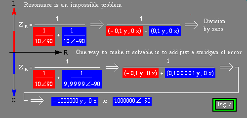
Perfect Resonance:
Resonant Frequency is defined as the frequency that capacitive
and inductive reactances are matched. Perfect resonance, the point
at which both capacitive and inductive reactances are matched,
and there is no resistive component what ever. This is ofcourse
a purely theoretical example, and it does, as you might expect
some pretty weird things. You end up with a problem that divides
by zero. However if we introduce a small, but insignificant amount
of error, we once again have a solvable problem. For the purposes
of this example I will shift the frequency ever so slightly
higher, to get an ever so slightly lower capacitive reactance.
For the purposes of this example I will assume that for some
unexplained reason the inductive reactance remained
unchanged :-) this is not the sort of thing
that is likely to happen in any real circuit, but it makes the
math easier to follow.
-------------------------------------------
fig 7   Solve for parallel impedance

               1 @ 0 deg
        ----------------------------
           1 @ 0 deg     1 @ 0 deg
        ------------- + ------------
         10 @ 90 deg    10 @ -90 deg

                  0 y ,  1 x
        ----------------------------
        (-0.1y, 0x) + (0.1y, 0x)

     Result
     division by zero


                  1 @ 0 deg
        --------------------------------
         1 @ 0 deg         1 @ 0 deg
        -----------  +  ----------------
        10 @ 90 deg     9.9999 @ -90 deg


                  1 y , 0 x
        -----------------------------------
        (-0,1 y , 0 x) + (0,100001 y , 0 x)


     Result
     -1000000y, 0 x  or  1000000 @ -90 deg

-------------------------------------------
In the above example by reducing the capacitive reactance
just a tiny bit, thus making the problem solvable, we end
up with a capacitive reactance that has a magnitude of one
million ohms!
So what would have happened, had we reduced the inductive
reactance, instead of the capacitive reactance? Basically all
the numbers would have been pretty much the same, except
instead of the final result being a very very high capacitive
reactance, it would have been a very very high inductive
reactance, that is the sign of the Y coordinate would have
been + or in the case of Polar format the angle
would have been + also indicating a inductance.
Notice what's happening here, as we get ever closer to the case
that causes division by zero, from the inductive side of the
vertical axis, we get results that rise ever higher in the
positive, eg. inductive reactance, and if you use a little
imagination, it's not hard to see infinity out there somewhere.
On the other hand approaching true perfect resonance
from the capacitive side of the vertical axis, we get results
that seem to be approaching an infinite negative number, eg. an
infinite capacitive reactance. So how do you make sense of this,
it seems as if true perfect resonance is this impossible to
imagine thing, the closer you get to it the higher it is, but
depending on which side of the fence you are sitting it's
either incredibly positive, or incredibly negative.
If this is a new concept to you, you're in for one those marvelous
moments in learning that leave your head in the clouds for days,
just thinking about the ramifications of it.
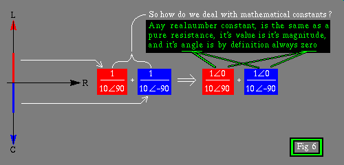
Listen up, what we are talking about here is ohms. The number
that Xc or Xl represent, is stated as ohms, yes it is reactive,
but in the absents of any other reference point, that is for
instance a resistance that might drop a voltage as a result
of current passing through the nearly infinite reactance, when
it does indeed reach infinity, it blocks all current, the series
dropping resistor, seeing no current, drops no voltage. If you
have no voltage to measure, you cannot know whither your series
reactance is inductive, or capacitive. It may seem like an
incredible leap of faith to simply assign a phase of zero to it
and be done with it, but under the circumstances, the calculations
won't know the difference. Even more to the point, when circuits
in any real world setting do things like having their impedances
start shooting up towards infinity, at some point you have to
start taking into account things like frequency turbulence of the
generator, essentially wobbling back and forth across the
frequency of true perfect resonance, causing the tuned circuit to
go from one extreme to the other, and you sitting there with
your Oscilloscope, trying to measure zero volts, and determine
what phase you are reading, is pointless. In other words
the very thing that division by zero prevents you from doing, is
also unnecessary. Long before true resonance reaches infinite
reactance other factors become so dominant that the notion of
whither it is capacitive, or inductive, is not only incalculable,
it cannot be determined experimentally with the best lab
equipment money can buy. The nearer you get to true perfect
resonance less you can say with any certainty which type of
reactance it is, you know it is in reality one or the other, it
has to be, it's just that you cannot know which, because of the
sea of noise. Strange to think of how the sign of a number that
is nearly infinite, can be drowned out by insignificant background
noise, but that is exactly what we have here. In addition there are
radiant losses, the signal itself radiates into space, this
mostly resembles a pure resistance, and let's not forget the
internal resistance of the generator, and the current sensing
resistor we are using to measure the phase, oh and did I mention
that air has resistance, yes air's resistance is pretty high, but
we are after all talking about a reactance of infinity, and at
infinity, air can scarcely compete with it's minuscule, multi-tera
ohm per cubic unit coefficient of resistance. All of these effects
are so small, that they defy lab measurement as well. So in a
practical sense, arbitrarily setting the phase of the infinite
reactance to zero, as a conceptual crutch, is not as far fetched
as it first appears to be.
In figure 8, and 9 I show another example of resonance with enough
true resistance to make for a circuit, that while it fits the
definition of resonance, Xc = Xl, is of such low Q eg. quality,
it barely fits the definition in any practical sense. It does
however provide me a way to give more detail to setting up the
problem of series parallel impedance, using as example the
reciprocal, of sum of reciprocals formula that you learned for
parallel resistors in
lesson 007 Series Parallel
earlier in this course. This example does not push the limits of
your scientific calculator's numerical precision, so the results
should be very close when you perform the exercise on your
calculator. Remember to follow the steps carefully, and watch those
signs.
-------------------------------------------
fig 8   Solve for series parallel impedance

  Step one: solve for the series
  resistor and inductor

  6 ohm pure resistance + plus 10 ohm
  inductive reactance

  (0 y , 6.0 x) + (10.0 y , 0 x)
  = (10.0 y , 6.0 x)

  Step two: Convert the series impedance of
  the inductor, resistor combination into
  Polar coordinates suitable for solving
  for the reciprocal.  Note: taking the
  reciprocal is essentially division.

  11.6619 @ 59.0362 degrees

  Step three: Now we set up the rest of the
  problem to solve for the parallel
  combination impedance of the capacitor,
  and the series, combination of the
  resistor, and inductor.


               1 @ 0 deg
  --------------------------------------
    1 @ 0 deg           1 @ 0 deg
  -------------- + ---------------------
   10 @ -90 deg    11.6619 @ 59.0362 deg


fig 9   This problem continues

  Step four: solving for the two lower
  reciprocal terms yields

                 1 @ 0 deg
  -----------------------------------------
  0.1 @ 90 deg  +  0.0857493 @ -59.0362 deg

  Step five: convert those two terms back
  to Rectangular I.E. Y,X coordinate pairs
  suitable for addition

               0 y ,  1 x
  --------------------------------------
  (0.1y, 0x) + (-0.0735294y, 0.0441177x)

  Step six: compute the coordinate pair sum
  of the two bottom terms

               0 y ,  1 x
  --------------------------------------
        (0.0264706y, 0.0441177x)

  Step seven: convert back to Polar, eg.
  Magnitude, and Angle to get it into a
  form suitable for division

         1 @ 0 deg
  --------------------------
    0.0514496 @ 30.9637

  Step eight: carry out the division, that
  is solve the last reciprocal

  Result is 19.4364 @ -30.9637 deg

  or in rectangular form the same

  Result is -9.9999y, 16.666x

-------------------------------------------
In fig 10 I show a much more realworld example, and unfortunately
realworld examples do push the limits of a scientific calculators
numerical precision. It also demonstrates how tiny resistances in
realworld resonant circuits, become the dominant factor in the
resulting phase. Notice that the mild inductance of this circuit
at resonance, only 12 ohms Xl, pales in comparison to the true
resistance of 20,000 ohms the circuit appears to possess when at
resonance. Also notice that none of the initial components were
anywhere near 20,000 ohms. I urge you to run the numbers, as a
confidence builder, especially if you lack familiarity in this
area.
-------------------------------------------
fig 10  Solve for series parallel impedance

  Step one: solve for the inductor with its
  inherent series coil resistance

  0.22 ohm pure resistance + plus 100 ohm
  inductive reactance

  (100 y , 0 x) + (0 y , 0.22 x)
  = (100 y , 0.22 x)

  Step two: Convert the series impedance of
  the inductor, resistance combination into
  Polar coordinates suitable for solving
  for the reciprocal.  Note: taking the
  reciprocal is essentially division.

  100.000242 @ 89.87394949 degrees

  Step three: solve for the capacitor with
  its ESR, "effective series resistance"

  0.28 ohm pure resistance + plus 100 ohm
  capacitive reactance

  (-100 y , 0 x) + (0 y , 0.28 x)
  = (-100 y , 0.28 x)

  Step four: Convert the series impedance
  of the capacitor, ESR combination into
  Polar coordinates suitable for solving
  for the reciprocal.

  100.000392 @ -89.83957224 degrees

  Step five: Now we set up the rest of the
  problem to solve for the parallel
  combination impedance of the capacitor/w,
  ESR, and the coil/w inherent series coil
  resistance


               1 @ 0 deg
  -----------------------------------------
   /         1 @ 0 deg                  |
  |  -----------------------------    --+--
   \ 100.000392 @ -89.83957224 deg      |

             1 @ 0 deg            \
     ----------------------------- |
     100.000242 @ 89.87394949 deg /


fig 11  This problem continues

  Step six: solving for the two lower
  reciprocal terms yields

                 1 @ 0 deg
  -----------------------------------------
  ( 0.009999960953 @ 89.83957224 deg  +
    0.009999975858 @ -89.87394949 deg )

  Step seven: convert those two terms back
  to Rectangular I.E. Y,X coordinate pairs
  suitable for addition

               0 y ,  1 x
  --------------------------------------
  (   0.009999921 y ,  0.000028 x   +
     -0.009999951 y ,  0.000022 x  )

  Step eight: compute the coordinate pair
  sum of the two bottom terms

               0 y ,  1 x
  --------------------------------------
  -0.000000030 y ,  0.000050 x

  Step nine: convert back to Polar, eg.
  Magnitude, and Angle to get it into a
  form suitable for division

         1 @ 0 deg
  --------------------------
    0.00005 @ -0.034606647

  Step ten: carry out the division, that
  is solve the last reciprocal

  Result is 20000 @ 0.034606647 deg

  or in rectangular form the same

  Result is 12.0799978y, 19999.996x

-------------------------------------------
In fig 12 I show the first use of Ohms law to, in this case
compute the voltage of an element in a reactive circuit.
-------------------------------------------
fig 12  To solve for AC voltage, "E" across
        a resistor and across the series
        capacitor, you need to solve for
        current, "I" to do this, you need
        to solve for total impedance, "Z"

  Er = R I           Egen
              I = ----------    Zt = Xc + R
  Ec = Xc I           Zt

  Knowns:
  Egen = 10.0 volts rms
  Xc   = 3000 ohm @ -90 deg
  R    = 10000 ohm @ 0 deg

fig 13  This problem continues

  Step one: solve for the total impedance

Zt = (-3000 y , 0 x) + (0 y , 10000 x)
   = (-3000 y , 10000 x)

  Step two: use Zt to solve for the current

      Egen         (0 y , 10 x)
I  = -------  =  ---------------------
       Zt         (-3000 y , 10000 x)

             10 @ 0 deg
   = -------------------------
      10440.3 @ -16.69924 deg

   = 0.00095783 @ 16.69924 deg

  Step three: use I to solve for the
  voltage drop across the resistor

Er = R I
   = (10000 @ 0) x (0.00095783 @ 16.69924)

  Result:  Er = 9.5783 volts @ 16.69924 deg

  Step four: use I to solve for the
  voltage drop across the capacitor

Ec = Xc I
   = (3000 @ -90) x (0.00095783 @ 16.69924)

  Result: Ec = 2.8735 volts @ -73.30076 deg

-------------------------------------------
Your home work:
Sorry this section needs, examples that you can work out, and maybe a
book recommendation or two, but I haven't any yet, so tune in later.
Back to Learn Electronics
Next
The large print Giveth, and the small print Taketh away
CopyLeft License
Copyright © 2000 Jim Phillips
Know then: You have certain rights to the source data,
and distribution there of, under a CopyLeft License